3. Under the Hood: Dissecting Spatial Accessibility Analysis • spax

Okay, Time for Some Theory!

We’ve been avoiding this moment for two whole vignettes, but there’s no escaping it anymore - we need to talk about theory. Don’t worry though! Like any good recipe, spatial accessibility analysis is just a matter of combining simple ingredients in the right way.

Let’s peek under the hood of spax to understand:

How spatial accessibility is actually calculated
Why we chose certain approaches over others
How theory translates into actual code

The Recipe for Spatial Accessibility

At its heart, spatial accessibility tries to answer a deceptively simple question: “How easily can people reach the services they need?” This involves three key ingredients:

People who need services (demand)
Places that provide services (supply)
The effort needed to connect them (distance/time)

The Enhanced Two-Step Floating Catchment Area (E2SFCA) method, which spax implements, combines these ingredients in two steps:

Step 1: Service-to-Population Ratios

First, we calculate how much service capacity is available relative to potential demand. For each service location $j$ :

$R_j = \frac{S_j}{\sum_i P_i W_d(d_{ij})}$

Where:

$S_j$ is the service capacity (like number of doctors)
$P_i$ is the population at location $i$
$W_d(d_{ij})$ is a weight based on travel time/distance
$R_j$ is the resulting service-to-population ratio

Think of this like calculating the “doctor-to-patient ratio” for each hospital, but with a twist – patients are weighted by how far they have to travel.

Step 2: Accessibility Scores

Then, we look at it from the population’s perspective. For each location i:

$A_i = \sum_j R_j W_r(d_{ij})$

Where:

$R_j$ is the ratio we calculated in Step 1
$W_r(d\_{ij})$ is another distance-based weight
$A_i$ is the final accessibility score

This tells us how much service capacity people can reach, accounting for both distance and competition from other users.

Rasterized formulas: A Different Perspective

While these formulas are traditionally written in terms of points $i$ and $j$ , our raster-based implementation thinks in terms of surfaces (~every point $i$ simultaneously). Let’s rewrite these equations to better reflect how spax actually computes them:

Step 1: Service-to-Population Ratios Raster Form

$r_j = \frac{s_j}{sum(P \odot \mathsf{W_d}(D_j))}$

Where:

$P$ is the population density surface
$D_j$ is the travel time/distance surface from facility $j$
$\mathsf{W_d}$ is the demand-side weighting function
$\odot$ represents element-wise (Hadamard) multiplication
$sum()$ is the global sum over the entire surface
$s_j$ is the supply capacity at facility $j$
$r_j$ is the resulting ratio for facility $j$

Step 2: Accessibility Scores - Raster Form

$A = \sum_j r_j \mathsf{W_r}(D_j)$

Where:

$A$ is now a complete accessibility surface rather than point-specific values.
$\mathsf{W_r}$ is the ratio-side weighting function

This raster-based formulation:

Eliminates the need to iterate over demand points $i$
Takes advantage of efficient matrix operations
Better reflects how spax works with continuous surfaces

From Formulas to Functions

Let’s see how these formulas - both traditional and raster-based - translate into actual code with spax:

library(spax)
#> Error in get(paste0(generic, ".", class), envir = get_method_env()) : 
#>   object 'type_sum.accel' not found
library(terra)
library(sf)
library(tidyverse)

# Load our example data
pop <- read_spax_example("u5pd.tif") # Population density
hospitals <- hc12_hos # Hospital locations
distance <- read_spax_example("hos_iscr.tif") # Travel times

# Let's look at the basic components for one hospital
example_hospital <- hospitals[1, ]

# Plot the fundamental surfaces
par(mfrow = c(1, 3))

# Population surface (P)
plot(pop, main = expression("Population Surface" ~ (P)))

# Distance surface for facility j (D[j])
plot(distance[[1]], main = expression("Distance Surface" ~ (D[j])))

# Weighted surface (W[d](D[j]))
plot(calc_decay(distance[[1]], method = "gaussian", sigma = 30),
  main = expression("Weighted Surface" ~ (W[d](D[j])))
)

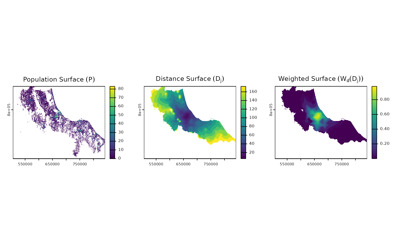
Each theoretical component becomes a raster operation:

Population Surface ( $P$ ): A single raster showing population density/
Distance Surfaces ( $D_j$ ): A stack of rasters, one per facility/
Weight Function ( $\mathsf{W_d}, \mathsf{W_r}$ ): Applied using calc_decay()

The real power comes in how spax chains these operations together efficiently. Rather than iterating over individual points, we: - Process entire surfaces at once - Use optimized matrix operations - Take advantage of parallel processing (via terra) where possible

Building Blocks: Core Operations in spax

Distance Decay: From Theory to Practice

Now that we understand the theory, let’s look at how we actually calculate those weight functions $W_d(d_{ij})$ or $\mathsf{W_d}(D_j)$ . The weight function’s job is simple - take a distance value and return a weight between 0 and 1. But how quickly should that weight decay with distance?

spax implements three classical decay functions (+ a binary decay), each offering different mathematical properties. Let’s align them at a common reference point (50% decay at 30 minutes) to see how they behave:

# Create example data with functions aligned at 50% decay at 30 minutes
example <- data.frame(x = seq(1, 160, 2))

example <- example |>
  mutate(
    gaussian_exp = calc_decay(x, method = "gaussian", sigma = 30),
    exponential_exp = calc_decay(x, method = "exponential", sigma = 0.0196),
    power_exp = calc_decay(x, method = "power", sigma = 0.1945)
  )

# Plot
ggplot(example, aes(x = x)) +
  geom_line(aes(y = gaussian_exp, color = "Gaussian")) +
  geom_line(aes(y = exponential_exp, color = "Exponential")) +
  geom_line(aes(y = power_exp, color = "Power")) +
  labs(
    title = "Distance Decay Functions",
    subtitle = "All functions aligned at 50% decay at 30 minutes",
    x = "Distance (minutes)",
    y = "Weight",
    color = "Function"
  ) +
  scale_y_continuous(limits = c(0, 1)) +
  theme_minimal()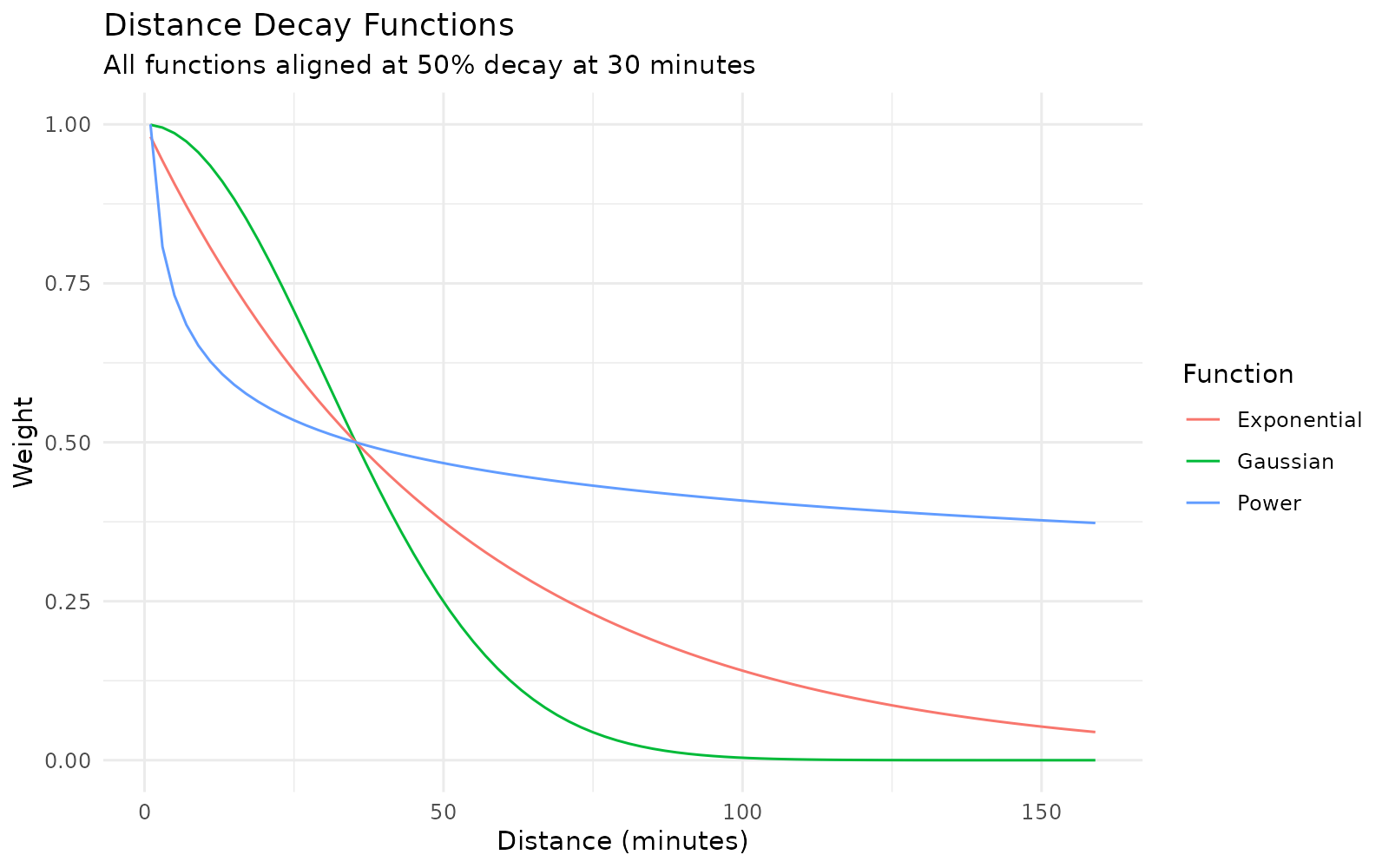

Each function offers a different mathematical perspective on how distance affects accessibility:

Gaussian decay ( $W(d) = e^{-d^2/(2\sigma^2)}$ ): Models accessibility like a bell curve, with the greatest change happening around that 30-minute mark/
Exponential decay ( $W(d) = e^{-\lambda d}$ ): Each additional minute of travel reduces accessibility by the same percentage/
Power decay ( $W(d) = d^{-\beta}$ ): Similar to exponential early on, but maintains higher weights at larger distances

Let’s see how these functions transform our distance surfaces:

# Extract one distance surface to explore
D_j <- distance[[1]] # Distance surface to our example hospital

# Calculate weights using different decay functions
gaussian_weights <- calc_decay(D_j,
  method = "gaussian",
  sigma = 30
)

exponential_weights <- calc_decay(D_j,
  method = "exponential",
  sigma = 0.0196
)

power_weights <- calc_decay(D_j,
  method = "power",
  sigma = 0.1945
)

# Visualize how different functions handle distance
par(mfrow = c(2, 2))
plot(D_j, main = "Original Distance Surface (D_j)")
plot(gaussian_weights, main = "Gaussian Decay")
plot(exponential_weights, main = "Exponential Decay")
plot(power_weights, main = "Power Decay")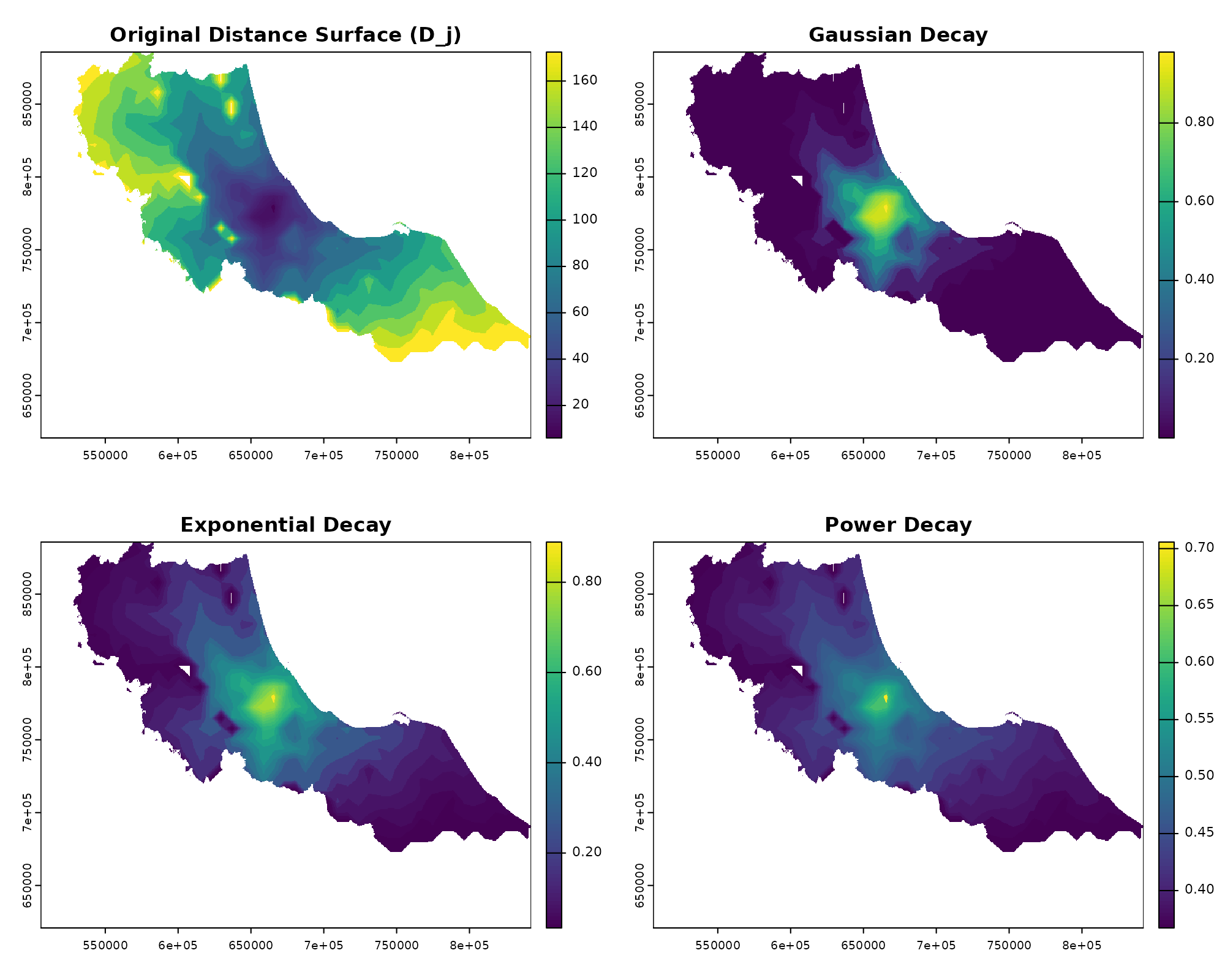

The beauty of spax’s raster-based approach is that these transformations happen all at once - every cell in our distance surface gets converted to a weight simultaneously. And because we’re using R’s vectorized operations under the hood, this works just as efficiently whether we’re looking at one facility or a hundred.

Want to create your own decay function? Any function that takes distances and returns weights will work:

# Custom decay combining distance threshold with Gaussian decay
custom_decay <- function(distance, sigma = 30, threshold = 40) {
  gaussian <- exp(-distance^2 / (2 * sigma^2))
  gaussian[distance > threshold] <- 0 # Hard cutoff at threshold
  return(gaussian)
}

# Use it just like the built-in functions
custom_weights <- calc_decay(D_j,
  method = custom_decay,
  sigma = 30,
  threshold = 60
)

# Plot
par(mfrow = c(1, 2))
plot(gaussian_weights, main = "Gaussian Decay")
plot(custom_weights, main = "Custom Decay\n(thresholded Gaussian)")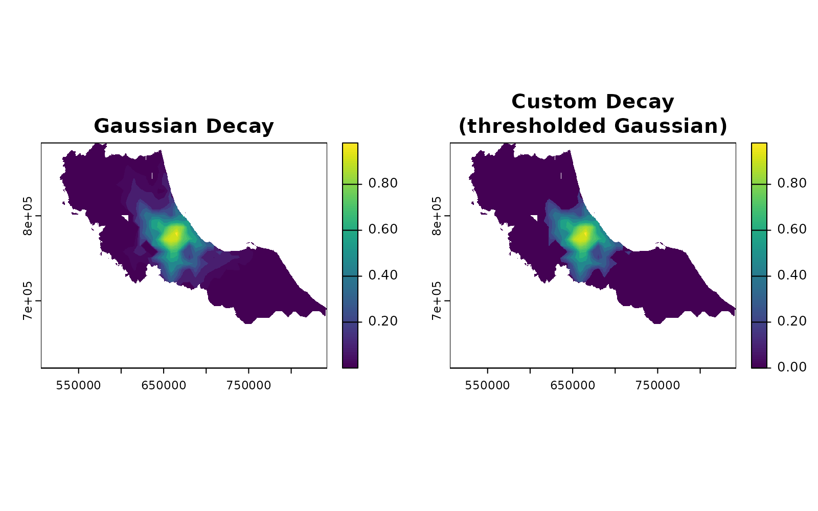

Managing Competition: Weight Normalization

Remember how we talked about counting patients in Step 1? Here’s where things get tricky. If we don’t handle overlapping service areas carefully, we might count the same population multiple times. This is where calc_normalize() and calc_choice() comes in:

# Create weight surfaces for two nearby facilities
W1 <- calc_decay(distance[[1]], method = "gaussian", sigma = 30)
W2 <- calc_decay(distance[[2]], method = "gaussian", sigma = 30)
facility_weights <- c(W1, W2)

# Compare different normalization approaches
standard_norm <- calc_normalize(facility_weights, method = "standard")
semi_norm <- calc_normalize(facility_weights, method = "semi")

# Visualize the effect of normalization
par(mfrow = c(2, 2))
plot(sum(facility_weights),
  main = "Raw Weight Sum\n(potential double-counting)"
)
plot(vect(bound0), add = TRUE)

# --
plot(sum(standard_norm),
  main = "Standard Normalization\n(sums to 1)"
)
plot(vect(bound0), add = TRUE)

# --
plot(sum(semi_norm),
  main = "Semi-normalization\n(prevents inflation)"
)
plot(vect(bound0), add = TRUE)

# Show where normalization matters most
overlap_areas <- sum(facility_weights) > 1
plot(overlap_areas,
  main = "Competition Areas\n(where normalization matters)"
)
plot(vect(bound0), add = TRUE)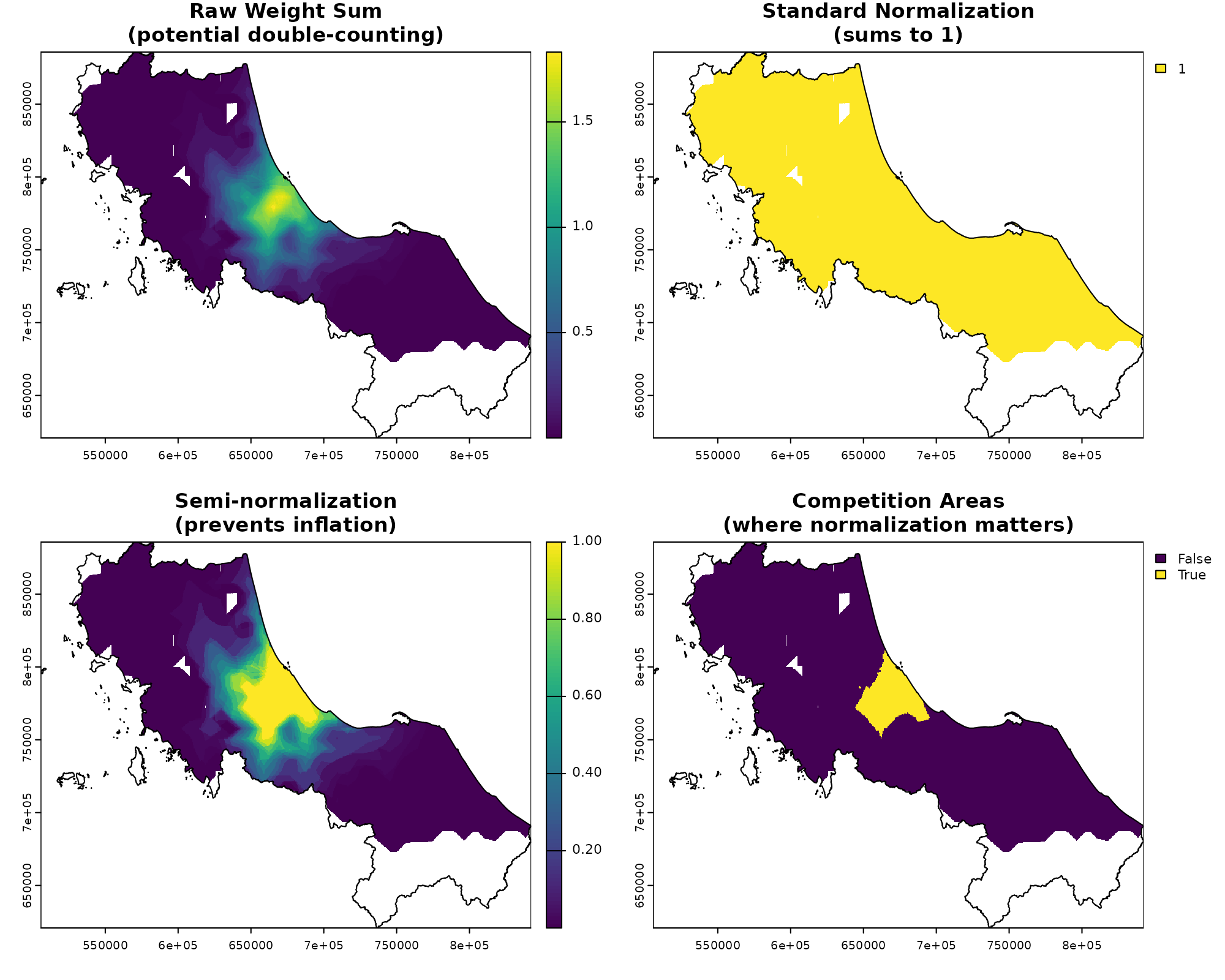

Think of normalization like adjusting a recipe when ingredients overlap. If two hospitals serve the same area:

Standard normalization: Forces weights to sum to 1, effectively splitting demand between facilities
Semi-normalization: Only adjusts weights where facilities actually compete (sum > 1)
No normalization: Allows double-counting, which might be appropriate for truly independent services

In our raster formulation, this becomes a simple operation on surfaces rather than complex point-wise calculations.

Spreading and Gathering: The Core Operations

Now for the real workhorses of spax: the spread_weighted() and gather_weighted() functions. These implement the summations in our formulas:

Traditional: $\sum_i P_i W_d(d_{ij})$ and $\sum_j R_j W_r(d_{ij})$
Raster: $sum(P \odot \mathsf{W_d}(D_j))$ and $\sum_j r_j \mathsf{W_r}(D_j)$

# Let's see these operations in action
# First, calculate potential demand for our facilities
potential_demand <- gather_weighted(
  pop, # Population surface (P)
  standard_norm, # Normalized weights (W_d)
  simplify = FALSE
)

print("Potential demand by facility:")
#> [1] "Potential demand by facility:"
head(potential_demand)
#>   unit_id weighted_sum
#> 1    c172     150186.5
#> 2    c173     139014.9

# Now calculate and spread accessibility
supply_ratios <- potential_demand |>
  mutate(
    ratio = hospitals$s_doc[match(unit_id, hospitals$id)] / weighted_sum
  )

print("Supply ratios:")
#> [1] "Supply ratios:"
head(supply_ratios)
#>   unit_id weighted_sum       ratio
#> 1    c172     150186.5 0.003475679
#> 2    c173     139014.9 0.002309104

accessibility <- spread_weighted(
  supply_ratios, # Facility-specific ratios (r_j)
  facility_weights, # Weight surfaces (W_r)
  value_cols = "ratio"
)

plot(accessibility, main = "Final Accessibility Surface (A)")
plot(vect(bound0), add = TRUE)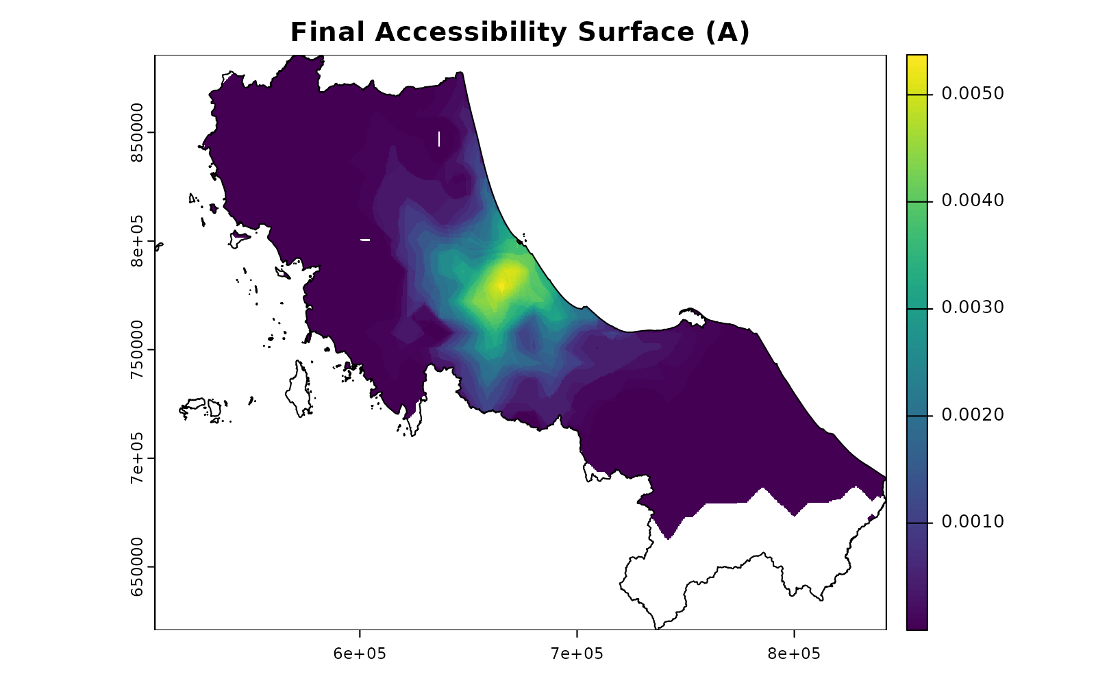

Think of these operations as: - gather_weighted(): Collects weighted values from a surface into facility-specific totals (a vector) - spread_weighted(): Distributes facility-specific values back across their service areas surface

Putting It All Together

Now that we understand each component, let’s see how spax_e2sfca() orchestrates them into a complete accessibility analysis. We’ll follow both the formula and the actual code:

The Complete Workflow

Traditional	Raster
Calculate $R_j = \frac{S_j}{\sum_i P_i W_d(d_{ij})}$ for each facility	Calculate $r_j = \frac{s_j}{sum(P \odot \mathsf{W_d}(D_j))}$ for each facility
Calculate $A_i = \sum_j R_j W_r(d_{ij})$ for each location	Calculate $A = \sum_j r_j \mathsf{W_r}(D_j)$ as a surface

Let’s see this step by step:

# Step 1a: Create distance decay weights
facility_weights <- calc_decay(
  distance, # Distance surfaces (D_j)
  method = "gaussian",
  sigma = 30
)

# Step 1b: Normalize weights to handle competition
demand_weights <- calc_normalize(
  facility_weights, # W_d(D_j)
  method = "standard" # Prevents double-counting
)

# Step 1c: Calculate potential demand for each facility
potential_demand <- gather_weighted(
  pop, # Population surface (P)
  demand_weights, # Normalized weights
  simplify = FALSE
)

# Step 1d: Calculate supply-to-demand ratios
supply_ratios <- potential_demand |>
  mutate(
    ratio = hospitals$s_doc[match(unit_id, hospitals$id)] / weighted_sum
  )

# Step 2: Calculate final accessibility surface
accessibility <- spread_weighted(
  supply_ratios, # Facility ratios (r_j)
  facility_weights, # Access-side weights (W_r)
  value_cols = "ratio"
)

# Visualize the final result
plot(accessibility, main = "E2SFCA Accessibility Surface")
plot(vect(bound0), add = TRUE)

Or we can let spax_e2sfca() handle all of this for us:

# The same calculation in one function call
result <- spax_e2sfca(
  demand = pop,
  supply = hospitals |> st_drop_geometry(),
  distance = distance,
  decay_params = list(method = "gaussian", sigma = 30),
  demand_normalize = "standard",
  id_col = "id",
  supply_cols = "s_doc"
)

plot(result, main = "E2SFCA Accessibility Scores")
plot(vect(bound0), add = TRUE)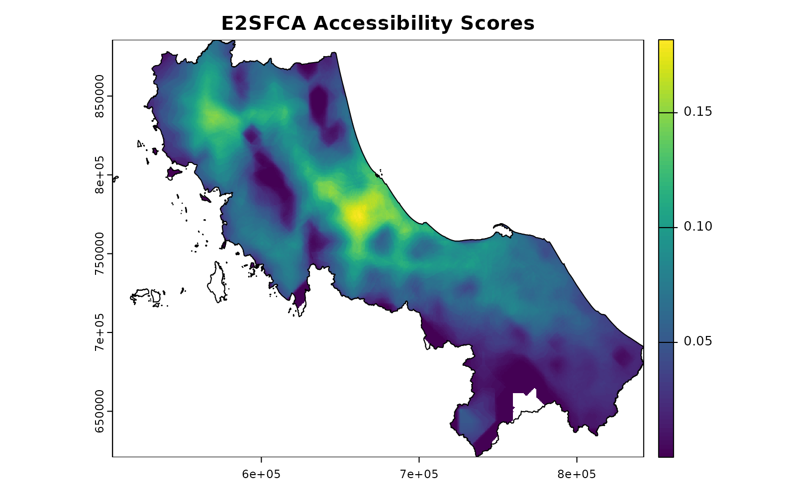

Understanding the Benefits

This modular design offers several advantages:

Flexibility: Each component can be customized:
- Different decay functions
- Alternative normalization approaches
Efficiency:
- Operations are vectorized across entire surfaces
- Memory usage is optimized for large datasets
- Parallel processing where beneficial
Transparency:
- Each step is clear and inspectable
- Results can be validated at any stage
- Intermediate outputs available for analysis
Extensibility:
- New components can be added easily
- Custom workflows can be built from basic pieces
- Alternative accessibility measures can be implemented

What’s Next?

Now that you understand how spax works under the hood, you might want to explore:

Understanding Raster Trade-offs: Learn about the memory and performance implications of our raster-based approach
Advanced Topics in Accessibility: Demand adjustment, normalization, and choice-based modeling [Coming Soon]