1. Getting Started with spax: A Healthcare Accessibility Case Study • spax

Getting Started with `spax`

Ever wondered how to measure whether people can actually reach the services they need? That’s where spatial accessibility analysis comes in. While there are many ways to approach this challenge, the spax package offers a fresh perspective with its raster-based tools.

What Makes spax Different?

Most accessibility tools work with points and distance matrices - think dots on a map connected by lines. spax takes a different approach:

Raster-First: At the expense of memory (lol), spax Built around continuous surfaces rather than discrete points, making it perfect for working with high-resolution population data or complex service areas
Modular Design: Chain together functions to build custom workflows - like LEGO bricks for spatial analysis
Performance-Focused: Optimized for large spatial datasets, because sometimes you need to analyze an entire region
Uncertainty-Aware: Because the real world isn’t deterministic, spax includes tools for Monte Carlo simulation and sensitivity analysis

The Building Blocks

Every spatial accessibility analysis needs three key ingredients:

Demand refers to the size and location of the population requiring services. It can be represented as a population density map or as aggregated values at administrative unit centroids (e.g., the number of elderly residents in each neighborhood).
Supply represents the capacity and location of service providers. This could be the number of doctors at each hospital, the number of seats available in schools, or even the stock of happy-hour cocktails at your favorite bar 🍸.
Distance: connects the dots between demand and supply. It defines the effort needed to bridge the two, whether through travel time or physical separation. Distances can be stored in matrices, calculated from coordinates, or derived from travel-time rasters, offering insights into the accessibility of supply to those in need.

Let’s see how these look in practice using our example dataset from Thailand’s Health Region 12.

Working with Example Data

📝 Data Note: The example dataset comes from Thailand’s Health Region 12, combining hospital records, Meta’s population density maps, and OSRM-computed travel times.

The package includes several integrated datasets (already lazy-loaded) that showcase healthcare accessibility analysis in action. Let’s load the required packages first:

library(spax) # For accessibility analysis
#> Error in get(paste0(generic, ".", class), envir = get_method_env()) : 
#>   object 'type_sum.accel' not found
library(terra) # For raster operations
library(raster)
library(sf) # For vector data handling
library(tidyverse) # For data manipulation + plotting

1. Understanding Demand

Our example uses under-5 population density data aggregated from Meta’s High Resolution Population Density Maps:

# Load the population density data
pop <- read_spax_example("u5pd.tif") # Under-5 population density

# Quick view of the data
print(pop)
#> class       : SpatRaster 
#> dimensions  : 509, 647, 1  (nrow, ncol, nlyr)
#> resolution  : 520.4038, 520.4038  (x, y)
#> extent      : 505646.5, 842347.8, 620843.7, 885729.2  (xmin, xmax, ymin, ymax)
#> coord. ref. : WGS 84 / UTM zone 47N (EPSG:32647) 
#> source      : u5pd.tif 
#> name        : tha_children_under_five_2020 
#> min value   :                      0.00000 
#> max value   :                     83.07421
res(pop) # each cell is ~520m x 520m
#> [1] 520.4038 520.4038

Let’s visualize this with our region boundary:

# Plot population density
plot(pop, main = "Under-5 Population Density")
plot(vect(bound0), add = TRUE) # Add region boundary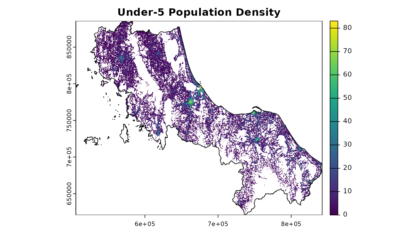

This raster shows us where children under 5 years old are located across the region, with brighter colors indicating higher density areas.

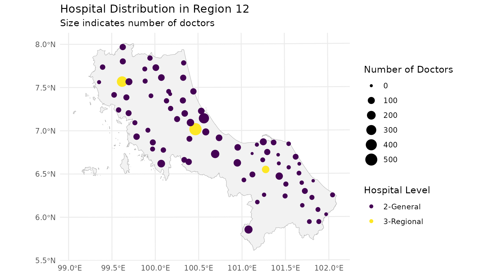
2. Exploring Supply

For healthcare supply, we have detailed information about hospitals (hc12_hos)

# Look at hospital data
head(hc12_hos)
#> Simple feature collection with 6 features and 10 fields
#> Geometry type: POINT
#> Dimension:     XY
#> Bounding box:  xmin: 659422 ymin: 744135 xmax: 715990.7 ymax: 824148
#> Projected CRS: WGS 84 / UTM zone 47N
#> # A tibble: 6 × 11
#>   id    hoslvl       bed s_doc s_dent s_nurse  s_hv d_pop_moph d_pop_moph_60
#>   <chr> <fct>      <dbl> <int>  <int>   <int> <int>      <dbl>         <dbl>
#> 1 c172  3-Regional   591   522     44     973     0          0             0
#> 2 c173  2-General    508   321     18     706     0          0             0
#> 3 c174  2-General     30    67      6      63     0          0             0
#> 4 c175  2-General     60    81      9     103     0          0             0
#> 5 c176  2-General     90   175     12     180     0          0             0
#> 6 c177  2-General     60    77      9     103     0          0             0
#> # ℹ 2 more variables: d_pop_moph_05 <dbl>, geometry <POINT [m]>

# Visualize hospital distribution and capacity
ggplot() +
  geom_sf(data = bound0, fill = "grey95", color = "grey70") +
  geom_sf(data = hc12_hos, aes(color = hoslvl, size = s_doc)) +
  scale_size_continuous(name = "Number of Doctors") +
  scale_color_viridis_d(name = "Hospital Level") +
  theme_minimal() +
  labs(
    title = "Hospital Distribution in Region 12",
    subtitle = "Size indicates number of doctors"
  )

3. Distance and Travel Time

The package includes pre-computed travel time data showing how long it takes to reach each facility:

# Load the travel time data
distance_raster <- read_spax_example("hos_iscr.tif")
distance_raster
#> class       : SpatRaster 
#> dimensions  : 509, 647, 77  (nrow, ncol, nlyr)
#> resolution  : 520.4038, 520.4038  (x, y)
#> extent      : 505646.5, 842347.8, 620843.7, 885729.2  (xmin, xmax, ymin, ymax)
#> coord. ref. : WGS 84 / UTM zone 47N (EPSG:32647) 
#> source      : hos_iscr.tif 
#> names       :  c172,  c173,  c174,  c175,  c176,  c177, ... 
#> min values  :   6.0,   3.0,   3.5,   4.0,   4.0,  11.0, ... 
#> max values  : 172.5, 172.5, 172.5, 172.5, 172.5, 172.5, ...
# Each layer represents travel time to a different facility


# Look at travel time to one facility
plot(distance_raster[[1]],
  main = "Travel Time to Hospital C1 (minutes)"
)
plot(vect(bound0), add = TRUE)
plot(hc12_hos[1, ], add = TRUE, pch = 16, col = "red")
#> Warning in plot.sf(hc12_hos[1, ], add = TRUE, pch = 16, col = "red"): ignoring
#> all but the first attribute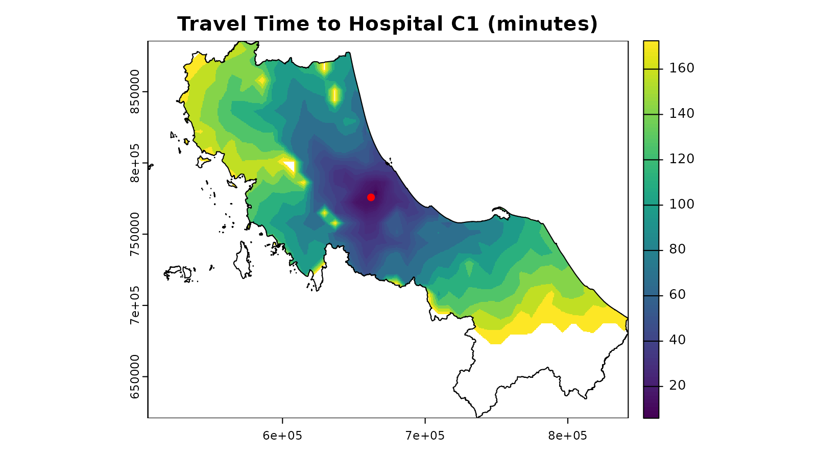

Quick Start: Basic Accessibility Analysis

Now that we understand our data, let’s put it all together for a basic accessibility analysis. We’ll use the Enhanced Two-Step Floating Catchment Area (E2SFCA) method to analyze access to doctors:

# Calculate accessibility scores
result <- spax_e2sfca(
  demand = pop, # Population density
  supply = hc12_hos |> st_drop_geometry(), # Hospital capacity
  distance = distance_raster, # Travel times
  decay_params = list( # How access decays with distance
    method = "gaussian",
    sigma = 30 # 30-minute characteristic distance
  ),
  demand_normalize = "standard", # Prevent demand inflation
  id_col = "id",
  supply_cols = c("s_doc", "s_nurse") # Analyze doctors and nurses
)

# Visualize the results
plot(result,
  main = c("Access to Doctors", "Access to Nurses"),
  fun = function() lines(bound0) # add region boundary
)

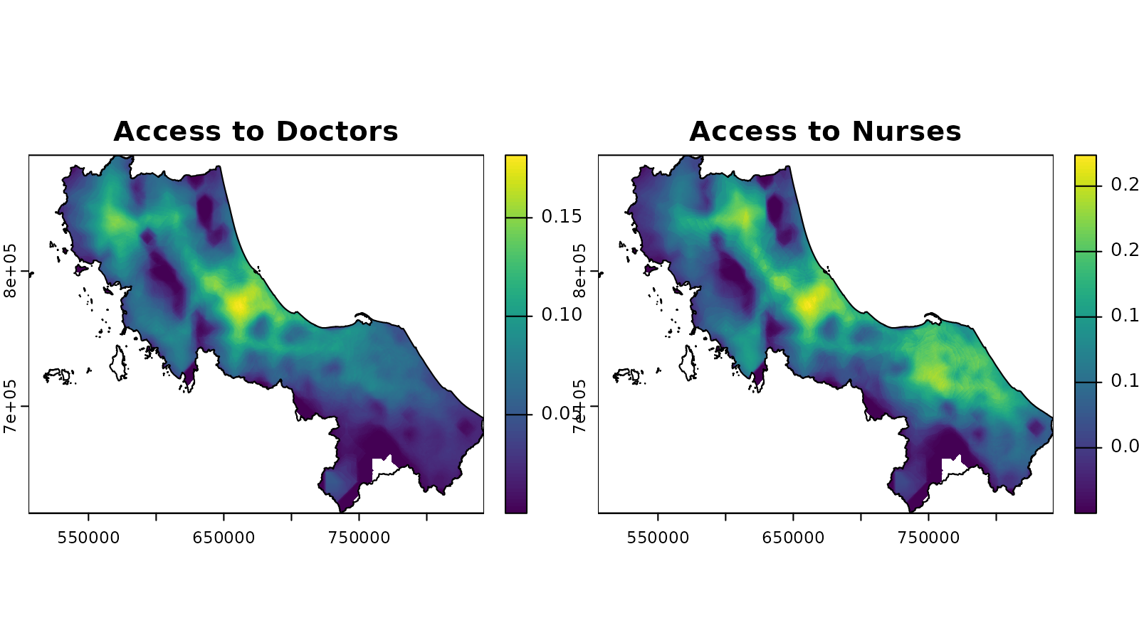
And that’s it! We’ve calculated accessibility scores for doctors and nurses across the region with the lighter colors indicating better access.

What’s Next?

This introduction just scratches the surface of what spax can do. For more advanced topics, check out: