Calculate Enhanced Two-Step Floating Catchment Area (E2SFCA) accessibility scores
Source:R/03-spax_e2sfca.R
spax_e2sfca.RdImplements the Enhanced Two-Step Floating Catchment Area (E2SFCA) method as proposed by Luo & Qi (2009). This method improves upon the original 2SFCA by incorporating distance decay effects and allowing for variable catchment sizes, providing more realistic measures of spatial accessibility to services.
Usage
spax_e2sfca(
  demand,
  supply,
  distance,
  decay_params = list(method = "gaussian", sigma = 30),
  demand_normalize = "identity",
  id_col = NULL,
  supply_cols = NULL,
  indicator_names = NULL,
  snap = FALSE
)
Arguments
- demand
SpatRaster representing spatial distribution of demand
- supply
vector, matrix, or data.frame containing supply capacity values
- distance
SpatRaster stack of travel times/distances to facilities
- decay_params
List of parameters for decay function:
method: "gaussian", "exponential", "power", or "binary"
sigma: decay parameter controlling the rate of distance decay
Additional parameters passed to custom decay functions
- demand_normalize
Character specifying normalization method:
"identity": No normalization (original weights)
"standard": Weights sum to 1 (prevents demand inflation)
"semi": Normalize only when sum > 1 (prevents deflation)
- id_col
Character; column name for facility IDs if supply is a data.frame
- supply_cols
Character vector; names of supply columns if supply is a data.frame
- indicator_names
Character vector; custom names for output accessibility layers
- snap
Logical; if TRUE enable fast computation mode (default = FALSE)
Value
A spax object containing:
accessibility: SpatRaster of accessibility scores
type: Character string "E2SFCA"
parameters: List of model parameters used
facilities: data.frame of facility-level information
call: The original function call
Details
The E2SFCA method enhances the original 2SFCA by introducing:
Step 1: For each facility j: * Weight demand points by distance decay: Wd(dij) * Calculate supply-to-demand ratio Rj = Sj/sum(Pi * Wd(dij))
Step 2: For each demand location i: * Weight facility ratios by distance decay: Wr(dij) * Calculate accessibility score Ai = sum(Rj * Wr(dij))
Key improvements over original 2SFCA: 1. Distance decay within catchments 2. Differentiated travel behavior in demand vs. access phases 3. Smoother accessibility surfaces 4. More realistic representation of access barriers
The method supports various distance decay functions and normalization approaches to handle different accessibility scenarios and prevent demand overestimation in overlapping service areas.
References
Luo, W., & Qi, Y. (2009). An enhanced two-step floating catchment area (E2SFCA) method for measuring spatial accessibility to primary care physicians. *Health & Place*, *15*(4), 1100-1107. https://doi.org/10.1016/j.healthplace.2009.06.002
See also
* [spax_2sfca()] for the original method without distance decay * [compute_access()] for more flexible accessibility calculations * [calc_decay()] for available decay functions
Examples
# Load example data
library(terra)
library(sf)
# Convert under-5 population density to proper format
pop_rast <- read_spax_example("u5pd.tif")
hos_iscr <- read_spax_example("hos_iscr.tif")
# Drop geometry for supply data
hc12_hos <- hc12_hos |> st_drop_geometry()
# Calculate accessibility with Gaussian decay
result <- spax_e2sfca(
demand = pop_rast,
supply = hc12_hos,
distance = hos_iscr,
decay_params = list(
method = "gaussian",
sigma = 30 # 30-minute characteristic distance
),
demand_normalize = "semi", # Prevent demand inflation
id_col = "id",
supply_cols = "s_doc"
)
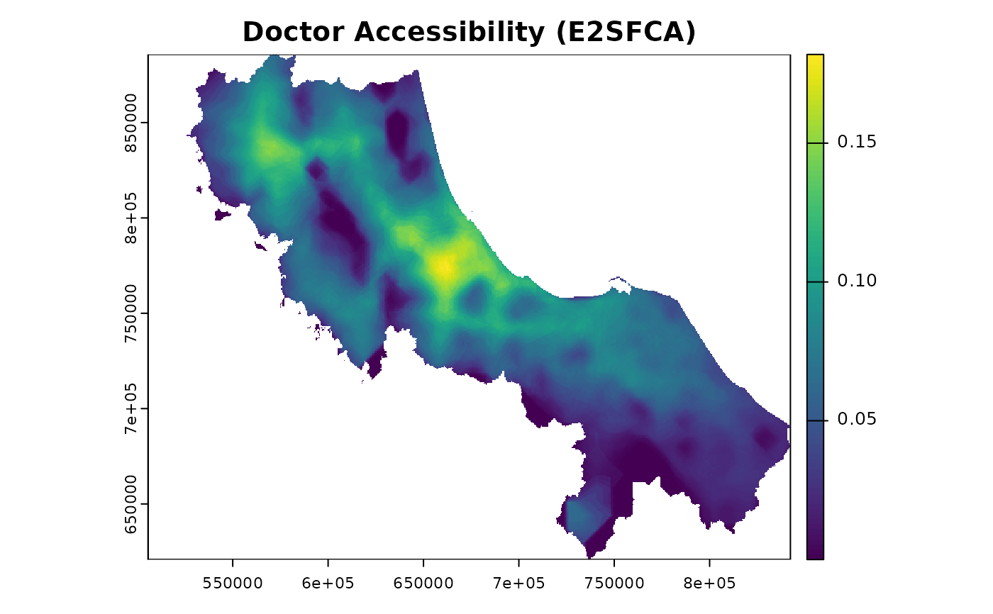
# Extract and plot accessibility surface
plot(result$accessibility, main = "Doctor Accessibility (E2SFCA)")
 # Access facility-level information
head(result$facilities)
#> id s_doc
#> 1 c172 522
#> 2 c173 321
#> 3 c174 67
#> 4 c175 81
#> 5 c176 175
#> 6 c177 77
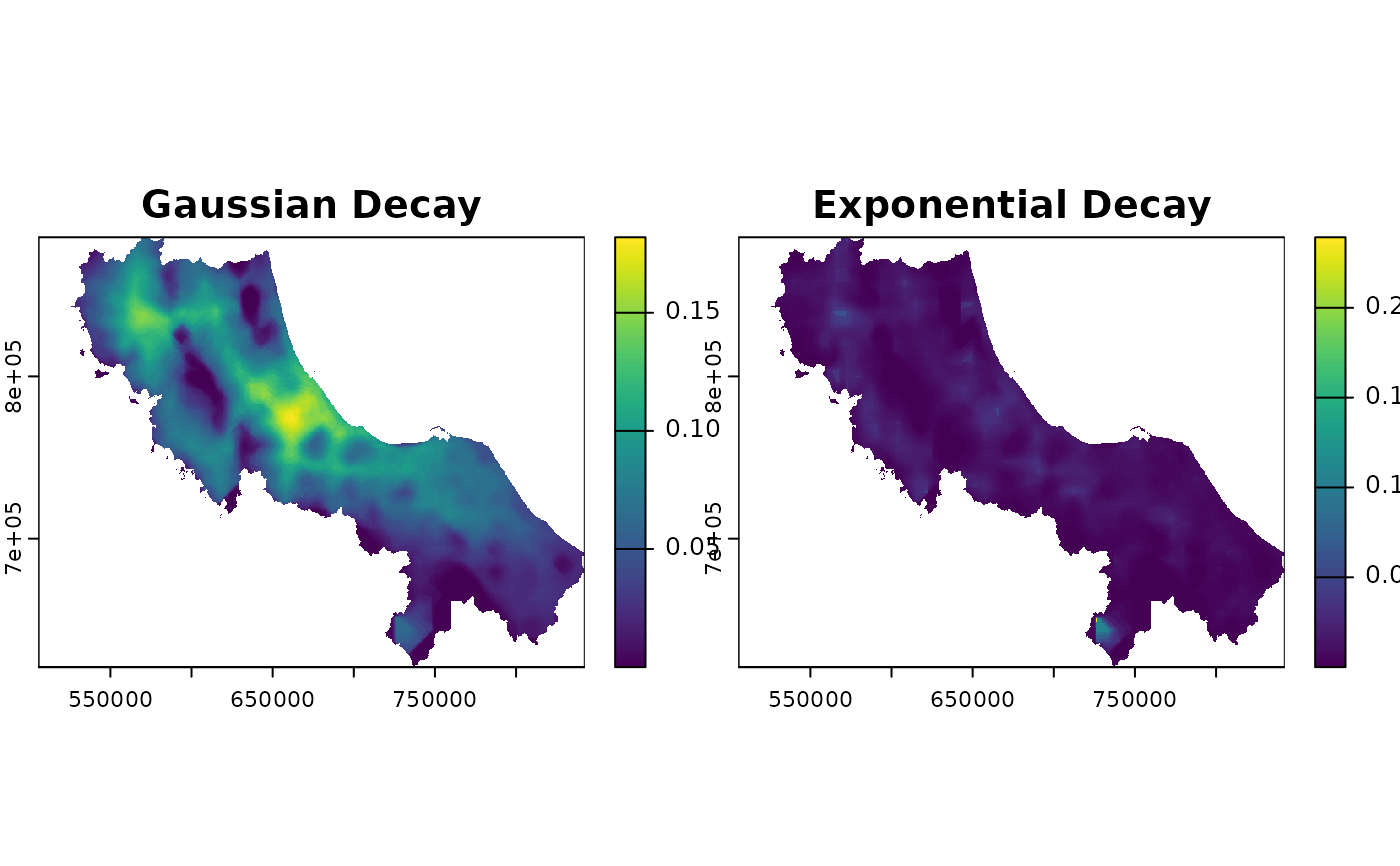
# Compare different decay functions
result_exp <- spax_e2sfca(
demand = pop_rast,
supply = hc12_hos,
distance = hos_iscr,
decay_params = list(
method = "exponential",
sigma = 0.1
),
demand_normalize = "semi",
id_col = "id",
supply_cols = "s_doc"
)
# Plot both for comparison
plot(c(result$accessibility, result_exp$accessibility),
main = c("Gaussian Decay", "Exponential Decay")
)
# Access facility-level information
head(result$facilities)
#> id s_doc
#> 1 c172 522
#> 2 c173 321
#> 3 c174 67
#> 4 c175 81
#> 5 c176 175
#> 6 c177 77
# Compare different decay functions
result_exp <- spax_e2sfca(
demand = pop_rast,
supply = hc12_hos,
distance = hos_iscr,
decay_params = list(
method = "exponential",
sigma = 0.1
),
demand_normalize = "semi",
id_col = "id",
supply_cols = "s_doc"
)
# Plot both for comparison
plot(c(result$accessibility, result_exp$accessibility),
main = c("Gaussian Decay", "Exponential Decay")
)